 |
 |
 |
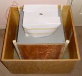
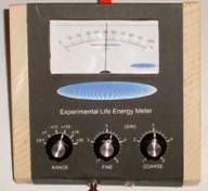
| Orgone Accumulator | Control and Monitoring | Detail of Sensor Area |
|---|
The entire accumulator is surrounded by a 1" air gap and this gap is surrounded by 3" of rock wool. A copper coil is located within the air space for heat control but is not used in the current experiment. The entire device is surrounded by a ¾" wooden enclosure. A second temperature probe is located in a cardboard cylinder (not shown) within the inner air space of the insulated chamber and at the same level as the accumulator probe. The temperature difference between the accumulator probe and the probe within the air space is To-T. A third temperature probe is located on top of the outer insulated wood box within a galvanized and grounded metal enclosure and is recorded as ambient temperature. This enclosure houses the Orgone Field Meter (Heliognosis LM3D), the dual plate vacuum tube and the Geiger counter. Also inside this enclosure is the signal conditioning electronics and the data acquisition system (Labjack U12). A laptop computer records all the data every minute in 24 hour periods from 9pm to 9pm. A precision temperature controller regulates the room temperature to 0.6 degrees Celsius using a forth temperature probe located on the top edge of the insulated wooden enclosure.
 |
 |
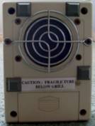 |
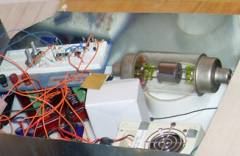
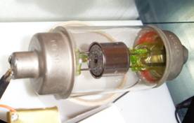
| Orgone Field Meter | Vacuum Capacitor | Geiger Counter |
|---|
The Orgone Field Meter used in this experiment is a Heliognosis LM3D with a 1 square inch brass electrode as the sensing plate located in the center of the galvanized enclosure. The galvanized enclosure is open at the top to allow for cosmic rays and atmospheric conditions to affect the sensors directly. The dual plate vacuum tube is a high vacuum glass capacitor with two cylindrical electrodes separated by a gap of about 1/8". This tube has a capacitance between the plates of 50pF. The capacitance of this tube is monitored using a precision capacitance meter circuit and then amplified to show the variation over time. Finally a Geiger Mueller counter with a 2" diameter pancake Geiger tube with a mica window faces towards zenith and is monitored for nuclear radiation counts per minute, primarily from cosmic rays. Signal conditioning electronics are employed to convert the raw signals into voltages that can be aquired by the Labjack data acquisition system.
 |
 |
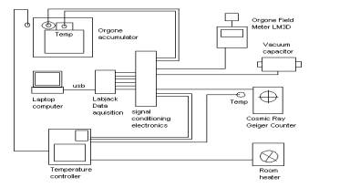
| Block Diagram of the Apparatus |
Labjack Data Acquisition System |
|---|
The Orgone accumulator is monitored to determine if heat accumulates within due to variations in atmospheric conditions. The Orgone field meter and the vacuum tube capacitor are measured to determine if atmospheric conditions influence the ability of the air space and vacuum space to hold charge. These two devices operate somewhat similarly to the electroscope. The Geiger Mueller counter primarily counts the number of incident cosmic rays from space. The atmosphere filters and modifies this radiation depending on its density and cloud cover.
The weather on March 1 was sunny with high pressure and very cold at -12 degrees C. The clear blue skies continued until March 5, when a low-pressure front moved in toward evening. The temperature had been generally rising over this period. March 6 was very warm (+16 C), unsettled with high winds and cloudy conditions until afternoon. Late in the afternoon the wind died down and the sky cleared completely and the pressure increased suddenly. The LM3D was operated on the x100 range with an additional 2x of amplification in the signal conditioning for a total of 200x of amplification. The capacitance of the vacuum was amplified 1000x and is shown as a voltage from the signal conditioning electronics. Looking at the graphs, the LM3D and vacuum tube both show a progressive decline through the entire period. The LM3D shows a distinct diurnal peak at 6 am and 3 pm each day. There is a small upward change in both the LM3D and vacuum capacitor on March 6 but much less dramatic than that shown for To-T. To-T is graphed in degrees Celcius vs. time. The To-T also shows a decline over the period finally rising suddenly at 4 pm on March 6 at about the moment that the low-pressure front moved out of the area. By the morning of March 7 a light rain had returned with overcast skies. To-T declined somewhat and leveled off as the unsettled weather continued until the end of this observation period. The atmospheric pressure had two minimums on the morning of March 6 and the evening of March 8. With the exception of the vacuum tube on the 6 (it was already close to a minimum), To-T, LM3D and the vacuum tube all showed minimums corresponding to the pressure minimums. To-T also shows diurnal variations typically peaking at around noon after a broad based rise through the night. Ambient temperature is graphed in degrees Celcius vs. time. Ambient temperature is shown with a typical variation of between 0.4 and 0.8 degrees C.
The cosmic ray background radiation was monitored over this period as is shown in the last graph below. Radiation is graphed as counts per minute vs. time. The average radiation was lower during sunny weather and higher during the cloudy and rainy period. In general, the cosmic ray count was pulsatory with major peaks approximately every 2.4 hours and minor peaks of about 12 minutes. It is interesting to note that the pulsation rate was higher during the cold sunny days at the beginning of the period. The skies were cloudless and no observable atmospheric phenomena could be seen to be responsible for the pulsation of the cosmic ray counts. Large longer pulses dominated during the unsettled and rainy days at the end of the period. It was the pulsatory nature of the cosmic ray counts that led to the possibility of determining the west-east movement of the pulsation discussed later in this report.
| Date (March, 2009) | 1 | 2 | 3 | 4 | 5 | 6 | 7 | 8 | 9 |
|---|---|---|---|---|---|---|---|---|---|
| Weather | sun clear |
sun clear & cold |
sun clear |
sun clear & warm |
sun -> cloud dry |
overcast wind & dry |
rain overcast |
rain wind |
light rain sunny breaks |
| Pressure (mB) | 1021 | 1022 | 1025 | 1021 | 1022-1012 | 1005-1011 | 1014-1010 | 1012-1004 | 1005-1019 |
| Humidity | 53% | 53% | 52-48% | 48% | 52-48% | 52-55% | 64-60% | 60-55% | 64-55% |
| Temperature (Celsius) |
-12 | -13 | -8 | -3 | 0 | 2 to 16 | 5 | 5 | 2 |
| Ion Count | n/t | -80 | -20 | 20 | -40 | 80 -> -50 | -2 | -50 -> 0 | 50 -> -10 |
Both detectors were 2" diameter pancake Geiger-Mueller tubes with mica windows. Both tubes were pointed towards zenith and the counts were primarily from incident cosmic rays. Count data was collected between March 29, 2009 and April 2, 2009. It had previously been determined that the cosmic ray flux was not constant and that the variation was as much as 10%. These variations had a consistent wavelike nature with periods of 12 minutes, 2.4 hours and long-term variations of about 1.5 days. Below is shown the Oakville data from March 5 to March 6 with a time average of one hour to highlight the approximate 2.4 hour wave cycle:
Data from James DeMeo’s lab in Ashland, Oregon was graphed in a similar fashion and shows the same wave phenomena. Counts per minute for February 27 to 28, 2009 using Rad50:
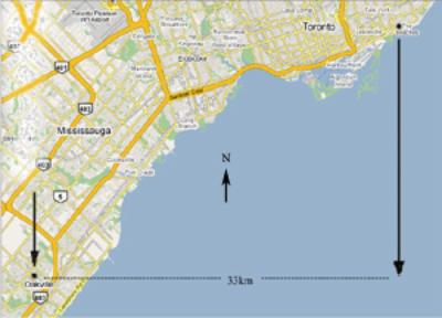
The count data from the Oakville and Beaches locations were graphed to look for similar patterns and to determine the time delay between the two observation points. The patterns lined up and indicated that the atmospheric wave pattern took 8 hours to travel from Oakville to the Beaches location. The speed of the wave-front is then 4.1km/hr in the west to east direction. The illustration below shows the graphed data from the two locations with a 7 hour moving average. Short-term peaks with a period of about 5 hours are actually two 2.4 hour peaks averaged together.
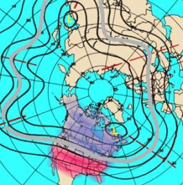
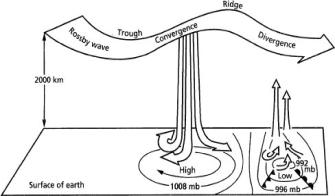
Melvyn A. Shapiro and Alan J. Thorpe5 have reported that the upper atmosphere has pressure variations with a group velocity that moves from west to east: the phenomena is known as Rossby wave effects, which travel on average at 97.7 km/hr at 45 degrees North latitude6. Since the observed wave formation is well below the Rossby wave speed range, it is unlikely that Rossby waves are the cause of the observed effect. Wind speed at ground level is about 20km/hr on average in March and is also unlikely to be the cause. An example of a Rossby wave diagram is shown below:
The cosmic ray data has revealed the interesting fact that it fluctuates with a period of about 2.4 hours. This period can increase and decrease and may have a relationship to the atmospheric conditions. Over a 5 day period, the cosmic ray pulsation is seen to travel in a west-east direction with an average speed of 4.1 km/hr. This result appears to be significantly smaller than that due to Rossby waves. Even in clear blue cloudless skies, the pulsation continues in a similar fashion as on rainy or overcast days. Therefore it is not due to varying densities of cloud cover. Future research will hopefully provide an answer to the true nature of this atmospheric wave.